The Mathematics of Deep-learning Optimisations- part 1
| Date: March 3rd, 2024 | Estimated Reading Time: 10 min | Author: Charlie Masters |
Table of Contents
I. The Objective of Machine Learning Algorithms
1. Defining the Loss Function
Explains the mathematical representation and importance of the loss function in ML algorithms.
2. Visualizing the Iterative Process
Describes how machine learning models iteratively adjust weights to minimize the loss function.
II. Gradient Descent
1. Concept and Formula
Introduction to the concept of gradient descent and the fundamental formula used for parameter updates.
2. Types of Gradient Descent
Discusses the different types of gradient descent: Batch, Stochastic, and Mini Batch.
a. Batch Gradient Descent
Covers the mechanics, advantages, and disadvantages of using Batch Gradient Descent.
b. Stochastic Gradient Descent
Details on how Stochastic Gradient Descent works, including its benefits and limitations.
c. Mini Batch Gradient Descent
Explains what Mini Batch Gradient Descent is and its significance in deep learning training.
III. Role of an Optimizer
Discusses the critical role optimizers play in enhancing the efficiency and effectiveness of training deep learning models.
IV. Types of Optimizers
Provides an overview of various optimizers like Momentum, Nesterov Accelerated Momentum, ADAM, NADAM, ADAGRAD, and RMSProp.
V. Example: The Colorization Problem
A practical example illustrating the application of discussed optimization techniques in a colorization task.
Over the course of this post, I will start to explain the purpose of algorithmic machine learning and the roles played by gradient decent in achieving this. We will also cover the mathematics of optimisation hyperparameters including Nestarovian momentum, Adagrad, Adadelta, RMSProp, Adam and NAdam and SGD.
In this Section I will explain the need for optimizers arising from the computational intensity of deep learning, and begin to go through some different types of optimizer that arise from models of gradient decent.
The objective of Machine Learning algorithm
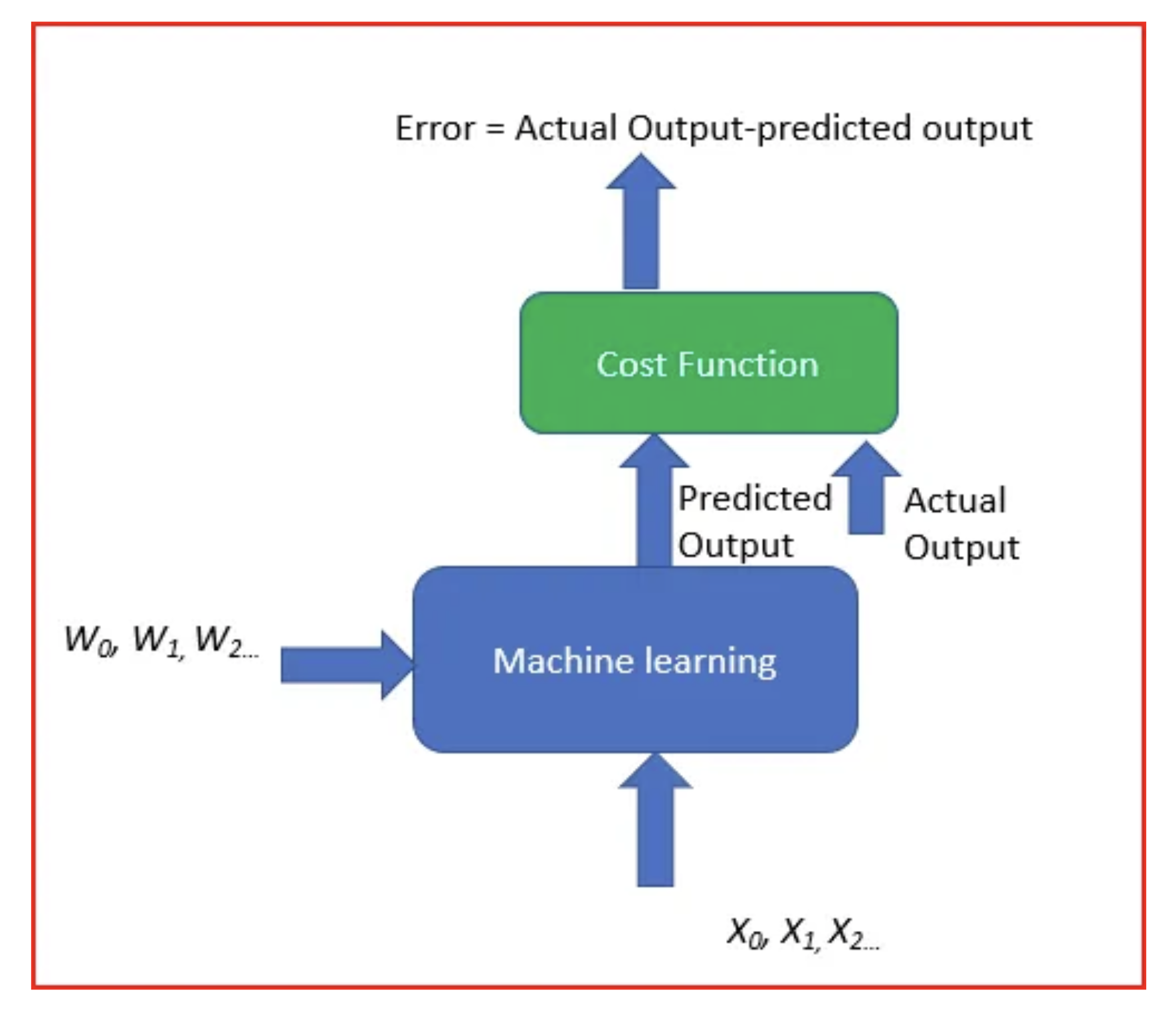
Machine learning algorithms are, in essence, a trial and error process of approaching a realistic model of data to attain a goal. This is typically done by reducing the difference between the predicted output and the actual output. The modelling of the differential between these two factors can be displayed by a Cost function(C) or Loss function, which are typically convex functions and thus follow the following definition:
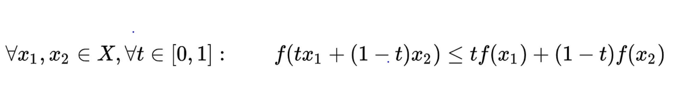
From this we can see that C approaches a local minimum in a vector space where it is minimised. Our strive for accurate models leads us to minimise the cost function by finding the optimum values for weightings, whilst still having the algorithm generalise well- lending itself to previously unseen useful predictions
To achieve this goal, we iterate our learning model with different weights to trend towards minimising cost. This is gradient decent.
Gradient Descent
Gradient descent is an iterative machine learning optimization to minimise the absolute value of the cost function. This will to maximise model accuracy.
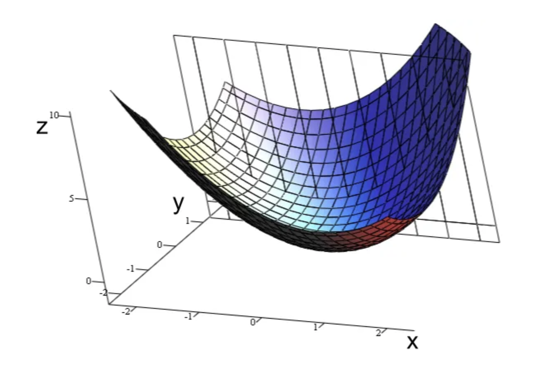
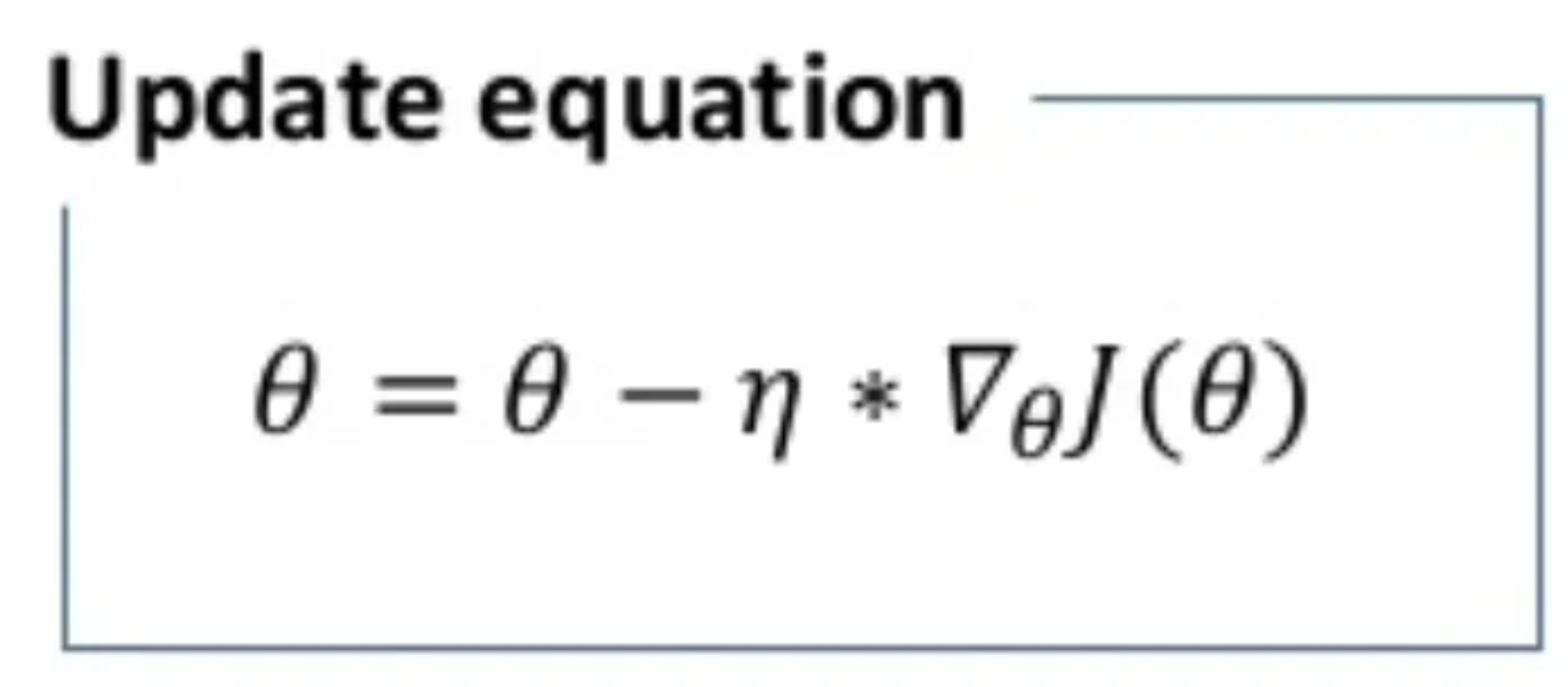
Gradient pertains to the direction of increase. As we want to find the minimum point in the “valley” we need to go in the opposite direction of the gradient. We update parameters in the negative gradient direction to minimize loss.
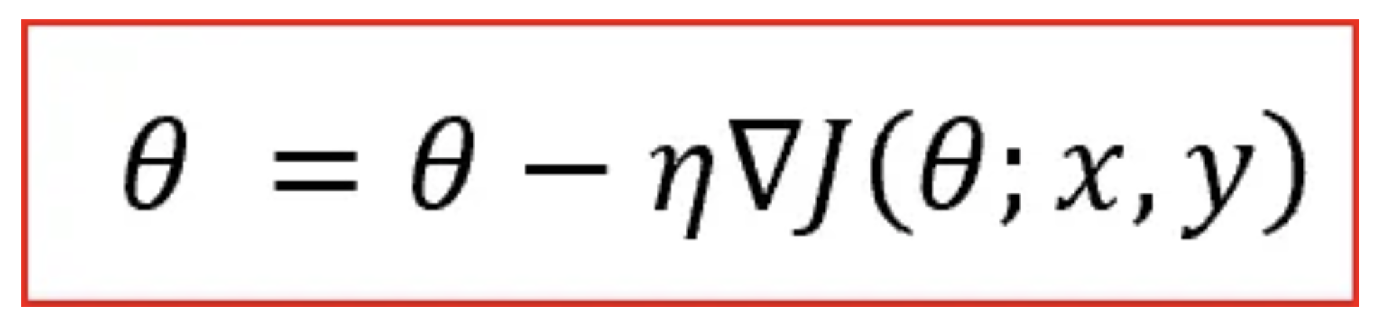
θ is the weight parameter, η is the learning rate and ∇J(θ;x,y) is the gradient of weight parameter θ in cartesian spacing.
Types of Gradient Descent
Gradient decent comes in many forms, each with their own benefits, drawbacks and use cases. Some prominent examples often used in deep learning are:
- Batch Gradient Descent or Vanilla Gradient Descent
- Stochastic Gradient Descent
- Mini batch Gradient Descent
I will assume understanding of the fundamental concept of gradient decent, but a coherent synopsis can be found here.
1 Batch Gradient Descent
In batch gradient decent algorithms the whole dataset is used in the computation of the cost function gradient for every epoch, and then weights are updated.
θ is the weight parameter, η is the learning rate and ∇θJ(θ) is the gradient of weight parameter θ in cartesian spacing.
Advantages of Batch Gradient Descent
- The theoretical analysis of convergence and weighting are conceptually simple to digest.
Disadvantages of Batch Gradient Descent
- Perform redundant computation for the same training example for large datasets
- Can be very slow and intractable as large datasets may not fit in the memory (with data lake based examples, whole batch may overload some computation package techniques, eg numpy array sizing limits.
Stochastic Gradient descent
In stochastic gradient descent we use discrete single training examples x(i) and labels y(i) to calculate gradients for the whole dataset before performing a single update.
This method can be considered as stochastic approximation of gradient descent optimization assuming loss function “smoothness”. Each epoch requires we shuffle the dataset so that we get a completely randomized dataset.
As the dataset is randomized and weights are updated for each single example, update of the weights and the cost function will involve stochastic noise, creating jagged function jumps as can be seen in the modelling later on.
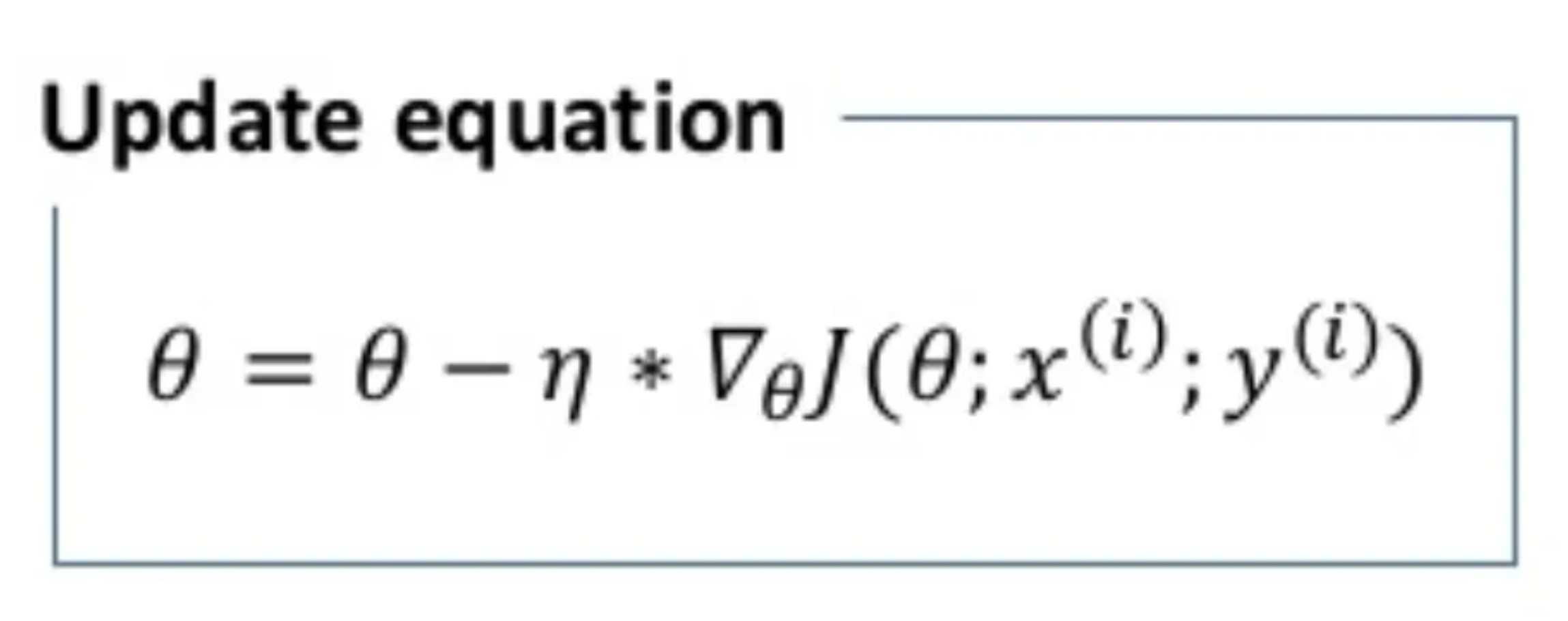
θ is again the weight parameter, η is the learning rate and ∇θJ(r) is the gradient of weight parameter θ in cartesian spacing where r is the spacing term for the weighting parameter with respect to the training example x and label y.
Advantages of Stochastic Gradient Descent
- Convergence of the decent of the loss function is far faster batch gradient descent.
- Redundancy is computation is removed as we take one training sample at a time for computation, stochastically approximating the gradient.
- Weights can be updated on the fly for the new data samples as we take one training sample at a time for computation
Disadvantages of Stochastic Gradient Descent
- As we frequently update weights, stochastic noise will lead the Cost function to fluctuate heavily. Although, in some use cases where the convergence of the G.D function is in fact only a “local” minimum, this will prove useful.
Mini Batch Gradient descent
Mini-batch gradient is a variation of stochastic gradient descent where instead of single training example, mini-batches of defined sample sizes are used.
Mini batch gradient descent is widely used and converges faster with less fluctuations. Batch size can vary depending on the dataset the model is training on.
As we take a batch with different samples, it reduces the noise which is variance of the weight updates and that helps to have a more stable converge faster.
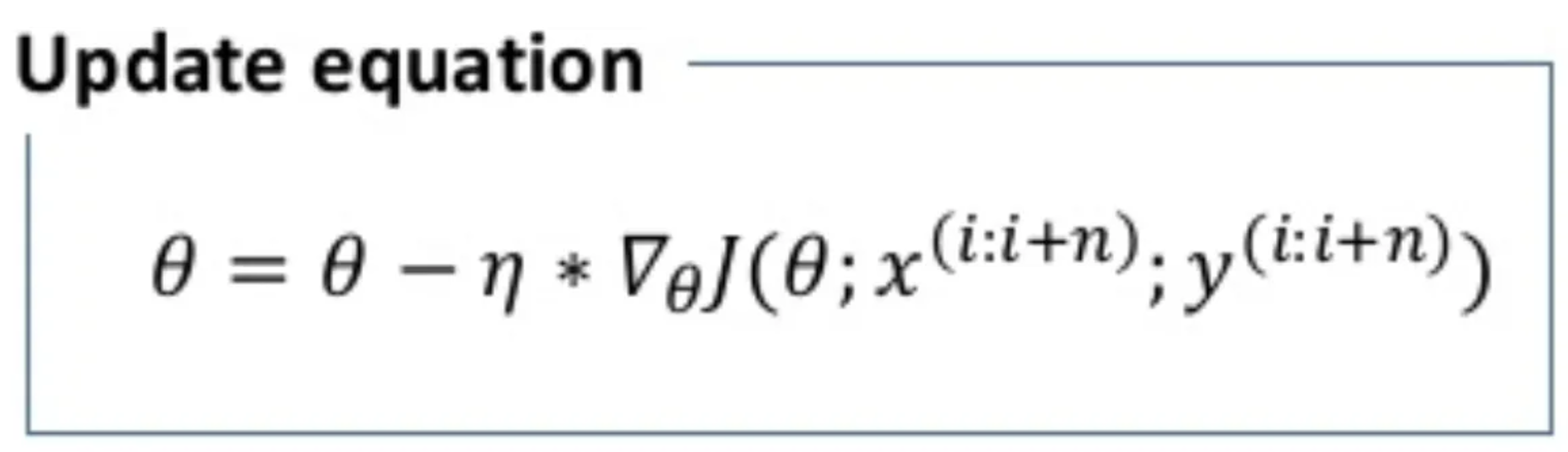
θ is again the weight parameter and η is the learning rate, ∇θJ(r) is the gradient of weight parameter θ in cartesian spacing where r is now the spacing term for the weighting parameter with respect to a batch size of size n iterated for the batches parameters and labels x(i) and y(i)
Advantages of Min Batch Gradient Descent
- Reduces variance of the parameter updates due to smaller stochastic noise spikes hence leading to stable convergence of the function.
- Speeds the “learning” of the model
- Helpful to estimate the approximate location of the actual minimum
Disadvantages of Mini Batch Gradient Descent
- Loss is computed for each mini batch and hence total loss needs to be accumulated across all mini batches
This should provide a brief road mapping of gradient decent for deep learning to illustrate later topics.
Role of an optimizer
An optimizer’s role is to reduce the exponential work and time required to train and get the weights of data points at each stage to minimize the loss function , show a better bias-variance trade-off and finally reduce computational time.
The importance of optimizers can be highlighted in deep learning by viewing the computational intensity of neural networks. Benchmarking off the CIFAR 100 dataset, the current highest rated neural network GPIPE with validation accuracy of 93% trains on a single 6-billion-parameter, 128-layer Transformer model.
Calculating this using linear operations without optimizers I hope would evidently not be exactly easy- and in cases where real time computation is required (think non reinforcement learning models of self driving cars, or swing trading RNN’s in financial markets), training these models would require time complexity that removes any applicability to real time tasks.
Types of Optimizers
The types of optimizer that we will consider are Momentum, Nestarov accelerated momentum, ADAM and Nestarovian ADAM (NAdam), ADAGRAD and RMSProp.
We will start by diving into Momentum and acceleration optimization in Part 2.